This series of posts will describe the use of the importance sampling estimator in the context of a recommender system. In this first post, we will explain what is a recommender system and how to formalize it as an instance of a contextual bandit problem.

The recommendation problem

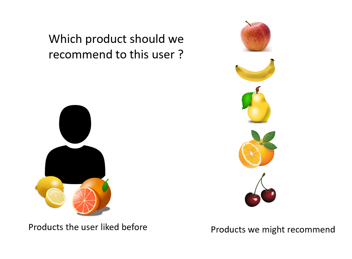
A recommender system is a system designed to propose to a user some content he may like, using the data available on this user. Some well-known use cases include choosing which movie to recommend to a user, knowing the list of previous movies he liked, or which products to advertise on a merchant website, knowing the past purchase of the user.

image-title-here

Predicting next organic view in the user session

The goal of the system is of course to recommend ‘relevant’ products to the user, so we need to define what is ‘relevant’. A widely used heuristic here is to define the ‘relevant’ products as the products the user is likely to view / purchase in the future, knowing the users’ current history of views / purchases. We can create logs of user histories removing the last item and then build models to predict this final item. This actually becomes a supervised learning problem.

a supervised learning problem

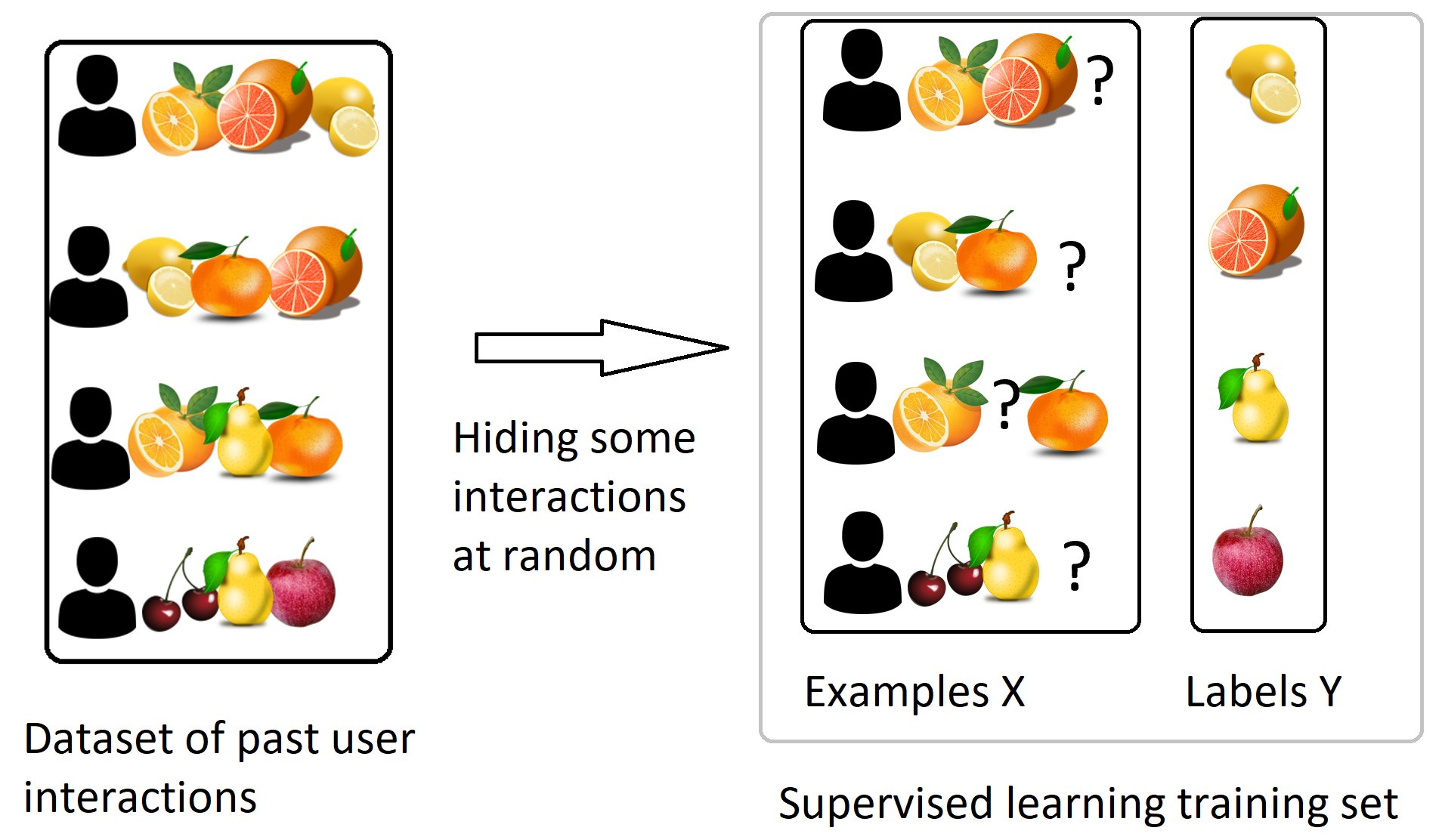
This supervised learning still requires some specific methods when the number of products is large. The most typical one is the ‘matrix factorization’ algorithm. You can find online many good descriptions of this algorithm, for example on wikipedia

Let’s note that the algorithms in this family only use the organic data on the user. Organic data sets involve logs of user behavior i.e. associations between items that are interacted with by the same user. Importantly these models do not use the logs of the recommender system (that contain information about past recommendations and if they were successful or not). This interaction (or bandit) data set is important - it tells us how well different recommendations in the past performed, but it is ignored by lots of traditional recommender systems literature. How can we leverage bandit data sets?

Optimizing the recommender system

Defining the goal of the recommender system

While predicting the next organic interaction of the user is a powerful heuristic, it is not actually the goal of the recommender system. This goal depends of course on the use case, but usually we can define it as retrieving the products the user is most likely to interact with when they are recommended. This interaction may be defined by clicks, conversion, likes, … depending on the exact use case. For example, at Criteo we commonly use “a click followed by a sale” to define a successful interaction with our recommender system. To simplify, we will just define it by “a click” in the following text, but keep in mind that the same methods could apply to any kind of reward.

The problem we are trying to solve is then the following: Knowing the history of the user, retrieve the recommendation which would maximize the probability that the user clicks.

This problem can be formalized as a contextual bandit.

Contextual bandits

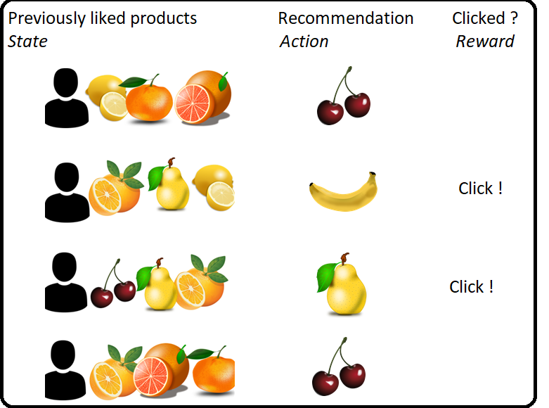
A contextual bandit problem is a setting where at the time step $i$:

the system observe a random state (sometime also called ‘query’ or ‘context’) $X_i$ . In the recommendation setting, $X_i$ will be the list of products liked by a user. The variables $X_i$ are assumed independent and identically distributed (iid)
it select an action $A_i$ for this user. Here $A$ will be the recommendation provided to the user.
it then receive a reward $R_i$ . Here the reward will be $1$ if the user clicks on the recommendation, and $0$ otherwise. The reward $R_i$ is assumed to depend only of the query and action $X_i$ and $A_i$ at the same timestep.

contextual bandit dataset

If you already know about Reinforcement Learning (RL), the definition of a contextual bandit should seem familiar. Actually, the only difference with RL is that we assume here that there is no dependency between the queries (or states) at different timesteps, whereas in RL the variable $X_i$ could depend on the previous state and action $X_{i-1}$ and $A_{i-1}$ . In other words, a contextual bandit is a simplified version of RL, where “episodes” are only of length 1.

Also note that assuming the independence between a recommendation $A_i$ and the future queries / reward is a hypothesis which is not perfectly true: in practice, we may observe the same user several times, and the recommendation we make to one user at a time $i$ may impact its query / reward when we see him again later. Making this assumption however removes many complications, so it can be worthwhile to work with it.

Policy

A policy $\pi$ is the mathematical object which describes how we choose the recommendation when we know the query $x$. It can be either deterministic, in which case it can be defined by a simple mapping $ x \rightarrow a $, associating to each state $x$ the recommended action $a$. Or more generally it can be stochastic: at each possible state $x$, we associate a probability distribution on the set of actions. We thus note, for a policy $\pi$, $\pi(a,x)$ the probability of choosing action $a$ when we are in state $x$.

Expected reward following a policy

When training models on a contextual bandit problem, the goal is to find the policy which maximizes the average reward:

$\hat{\pi} = Argmax_{ \pi } \mathbb{E}_X ( \mathbb{E}_{ A \sim \pi } ( \mathbb{E}( R | A = a , X = x )))$

Note that the optimal policy $\hat{ \pi}$ is usually deterministic: In each context, just choose the action which maximize the expected reward $\mathbb{E}( R | X=x, A=a) $.

However, it is usually a good idea to avoid fully deterministic policies. One of the main reasons is that a randomized policy allows us to keep some exploration on the different actions, and this is useful to learn how to improve the policy. It is also useful to evaluate a new policy, as we will describe in the next sections.

So how is this different from supervised learning?

Finding the best policy could be restated as follow:

for each query $x$, find the action $a$ which maximizes $ \mathbb{P}( C =1 | X = x ,A = a ) $

This might look like something which could be solved by some simple supervised learning, fitting a model to predict $ \mathbb{P}( C =1 | X = x ,A = a ) $ to the available data. So is there something more?

The first difference is that to learn the model you need to explore the different actions. If you always play the action you think is the best, you won’t get data on the other actions and will never learn that they might actually be better.
Second difference is that the classical supervised learning losses may be very ill-adapted to evaluate the performance of a model.

To understand better the difference, let’s look at a toy example. Let’s say that there are only two possible queries, 3 actions, and that we collected a dataset with the following probability of click.

Probability of click	Action a	Action b	Action c
query 1	0.5	0.55	no data
query 2	0.2	0.25	no data

Let’s look at a possible model:

model 1 output	Action a	Action b	Action c
query 1	0.52	0.52	0.52
query 2	0.22	0.22	0.22

This model would perform quite well according to metrics like ‘RMSE’. Indeed, it does a decent job at predicting the probabilities of click. However, it does not help to choose an action, as its prediction does not depend on the action!

Compare now to this other model:

model 2 output	Action a	Action b	Action c
query 1	0.35	0.4	0.35
query 2	0.35	0.4	0.35

This second model would perform worse according to RMSE than the previous one (because the values it outputs are quite far from the actual probability of a click). However, it does correctly pick action b over action a on both queries and is therefore more useful.

Let’s note also that the prediction on Action C does not impact at all the RMSE (because we have no data there), while it might actually perform totally differently.

All that being said, fitting a model predicting $ \mathbb{P}( C =1 | X = x ,A = a ) $ to the available data and choosing the best action according to this model can be a very strong baseline, especially when a bit of randomization is added to enforce some exploration. It is however not a great idea to select the model only based on classical supervised learning metrics.

In the next post, I will describe how we can build better offline metrics for contextual bandits. More specifically, we can build a metric which under some mild assumptions can estimate “how many clicks we would get if we were using the test policy”. Doesn’t it sound like the perfect metric?