Counterfactual reasoning with the Importance Weighting Estimator

This post explains how to perform offline evaluation of a new version of the system using the “importance sampling estimator”

Counterfactual reasoning with the Importance Weighting Estimator

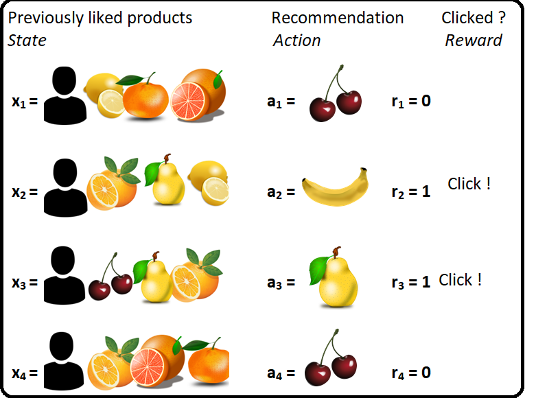
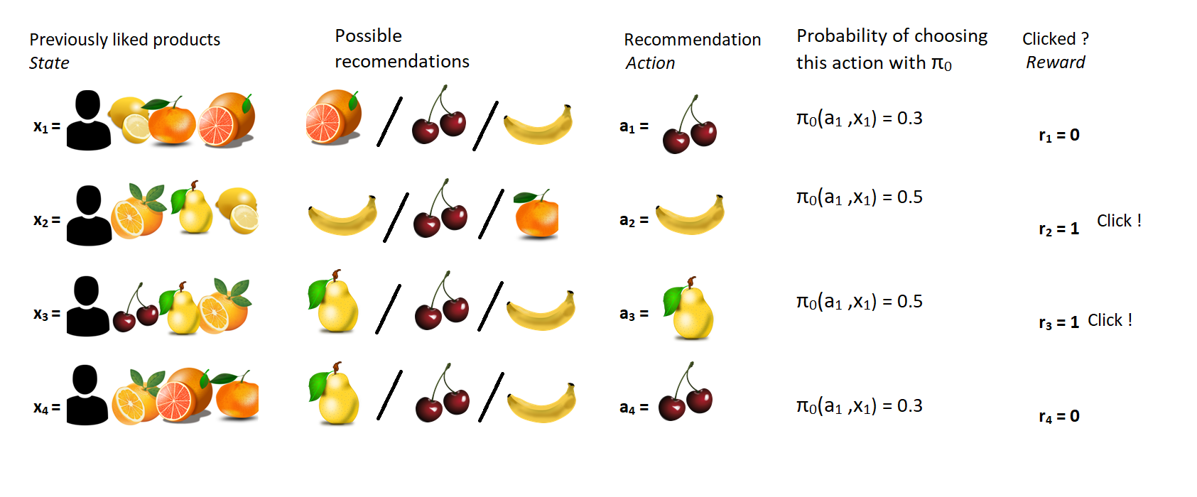
Let’s assume we have been collecting some dataset of our contextual bandit, using one policy $\pi_0$. We thus have a dataset $(x_i, a_i, r_i)$ where:

• $x_i$ are iid samples of the state X.
• $a_i$ is a sample from $\pi_0$ on state $x_i$
• $r_i$ is a sample of the reward when the state is $x_i$ and the action $a_i$

And let’s say we have a new algorithm, providing a new policy $\pi_{test}$. We would like to know how it performs. More precisely, we would like to know which total reward we would have got, if we had used $\pi_{test}$ instead of $\pi_0$.

Can we do that only from our offline data?

The surprising answer is ‘Yes, we can’, under some rather mild assumptions. More precisely, we will construct an unbiased estimate of how many clicks we would have got with test policy.

Let’s already state those assumptions:

• we are in a ‘contextual bandit’ setting. See the previous post for more details, but this mostly means that what is happening at a timestep $i$ does not depend on the other timesteps.
• the policy $\pi_0$ used to collect data must be stochastic and explore all the actions: for any state $x$ and action $a$, $\pi_0$ should play $a$ in state $x$ with a non $0$ probability.

Under those hypotheses, we can estimate the total reward we would have got when using $\pi_{test}$ with the ‘Importance Sampling Estimator’ (IPS), defined as follow:

$$ips := \frac{1}{n} \times \sum_\limits{ i \in {1...n} } \frac{ \pi_{test}(x_i,a_i) }{ \pi_0(x_i,a_i) } r_i$$

Let’s already try to interpret this formula:

• we are counting the clicks $r_i$
• each click is reweighted by the ratio $\frac{ \pi_{test}(x_i,a_i) }{ \pi_0(x_i,a_i) }$
• and we divide by $n$ to get a ‘ratio of clicks per user’

A simplified example

To get an intuition on why this formula would work, let us look at a simplified example, with only one single state $x_0$, and two actions, ‘red’ and ‘green’.

Let’s assume we collected some data with the following policy:

• $\pi_0(red,x_0) = 0.8$
• $\pi_0(green,x_0) = 0.2$

And that after applying this policy to 10000 users, we got a total of 1000 clicks after the cases when red was chosen, and 300 after green.

Let’s say we would like to test this new policy:

• $\pi_{test}(red,x_0) = 0.2$
• $\pi_{test}(green,x_0) = 0.8$

Can we tell which results to expect if we follow this new policy?

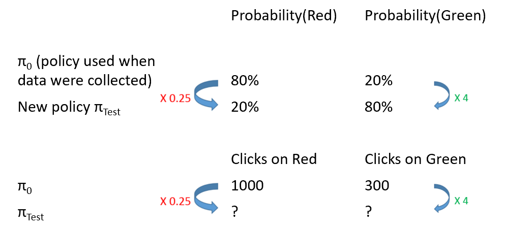
As the diagram suggests, the test policy chooses green $4$ times more often than $\pi_0$, so we may expect $4$ time more clicks on green. It also chooses red 4 time less often so we should expect 4 times less clicks on red.

The final answer is then: $$Clicks_{green} \times \frac{ \pi_{test}(green) } { \pi_{0}(green) } + Clicks_{red} \times \frac{ \pi_{test}(red) } { \pi_{0}(red) } = 300 \times \frac{ 0.8 }{0.2} + 1000 \times \frac{ 0.2 }{0.8} = 1450$$

We can see that the ratios $ \frac{ \pi_{test}(green) } { \pi_{0}(green) } = 4 $ and $ \frac{ \pi_{test}(red) } { \pi_{0}(red) } = 0.25 $ are quite intuitive to apply here, and that the final formula is exactly the $IPS$ estimator has defined above.

Note that this is correct because the choice of ‘red’ or ‘green’ were made at random, following a known policy $\pi_0$. It would not be correct anymore if the choice of red / green was depending on some other variables, and the “80% red, 20% green” was only the average on different users. In this case, such a reasoning would certainly not work any more and could lead to totally wrong conclusions, as for example in the case of Simpson’s paradox.

An unbiased estimator

We just estimated, from the data in this example, that using the $\pi_{test}$ policy we would have got 1450 clicks. Does it mean that we would observe exactly 1450 clicks if we had collected the data with $\pi_{test}$? Certainly not. This number of clicks with the test policy is a random variable, and we have only an estimator of its average. We will explain further why it is unbiased, which means the following: if we replayed infinitely many times the experiment we just did, which is:

• collect some data with $\pi_0$
• compute the estimator $ Clicks_{green} \times \frac{ \pi_{test}(green) } { \pi_{0}(green) } + Clicks_{red} \times \frac{ \pi_{test}(red) } { \pi_{0}(red) }$ on those data

We would get, on average on those experiments, the average number of clicks we would get with $\pi_{test}$.

Back to the general problem

Previous example suggests an interpretation for the weights $\frac{ \pi_{test}(x_i,a_i) }{ \pi_0(x_i,a_i) }$ They represent ‘how much more likely’ is action $a$ with $\pi_{test}$ than with $\pi_0$ in the context $x$. We will name this ratio the ‘importance weight’ and note it $w$:

$$w_i := w(a_i,x_i) := \frac{ \pi_{test}(x_i,a_i) }{ \pi_0(x_i,a_i) }$$

In the general case of course, the users may be all different, and the policy $\pi_0$ can depend on the user. How can it be unbiased in those conditions? To understand that, let’s first note that if we decrease the number of users in the previous experiment, we get (of course) a worse estimator because the variance increases, but it still remains unbiased. In particular, it is unbiased even when there is a single user!

So in the general case, we get on each user an unbiased (but very high variance) estimator of what would happen when using test policy for this user. By summing those estimators on all users, it is still unbiased (for the population of users), and the relative variance (hopefully, more on that later) goes down.

Proof of unbiasedness

Following the usual convention, I will use upper case letters ($X$, $A$, $IPS$, …) for random variable and lower case ($x$, $a$, $ips$, …) to denote a realization from a random variable.

Expected reward when using the test policy

Let’s first define the “expected reward when using the test policy $\pi_{test}$” , noted $\mathbb{E}_{\pi_{test}}(R)$:

It is the expectation of the outcome of the following random experiment:

• draw a random user state $X$, from the environment.
• draw an action $A$ following the policy $\pi_{test}(x)$.
• draw a sample of the reward $R$ for this (state, action), and return its value.

Using the chain rule, we can write: $$\mathbb{E}_{\pi_{test}}(R) = \sum_\limits{x} \mathbb{P}(X=x) \sum_\limits{a} \pi_{test}(A=a | X=x) \mathbb{E}( R | A=a , X=x )$$

Let’s emphasis what we know in this formula:

• $X$ comes from an environment that we do not control: we do not know the value of $\mathbb{P}(X=x)$.
• $\pi_{test}(A=a | X=x) $ depends on the policy $ \pi_{test} $ we want to try. We typically have defined ourselves this policy, so we should be able to compute explicitly this number.
• $ \mathbb{E}( R | A=a , X=x ) $ describes how a user in a state $x$ reacts to a recommendation $a$. This is not known either.

IPS estimator

Let’s then notice that the value $$ips := \frac{1}{n} \times \sum_\limits{ i \in {1...n} } w(a_i,x_i) \times r_i$$ computed on our dataset is a sample of the random variable $$IPS := \sum_\limits{ i \in {1...n} } w(A_i,X_i) \times R_i$$

What we would like to prove now is that $IPS$ is an unbiased estimator of $\mathbb{E}_{\pi_{test}}(R)$, in other words that $$\mathbb{E}(IPS) = \mathbb{E}_{\pi_{test}}(R)$$

So let us write its expectation:

$$\mathbb{E}(IPS) = \frac{1}{n} \times \sum_\limits{ i \in {1...n} } \mathbb{E} ( w(A_i,X_i) \times R_i )$$

since all samples are identically distributed,

$$\mathbb{E}(IPS) = \mathbb{E} ( w(A_1,X_1) \times R_1 )$$

Using the chain rule, we can now decompose the expectation on the different random variable (note that $A_1$ from our sample was following the policy $\pi_0$ ):

$$\mathbb{E}(IPS) = \sum_\limits{x} \mathbb{P}(X_1 = x) \sum_\limits{ a \in actionsSet } \mathbb{P}(A_1 = a | X_1 =x) \times w(a,x) \times \mathbb{E}( R_1 | A_1 = a , X_1 = x )$$

I kept the indices $X_1$, $A_1$ to remind that those are samples from our dataset. This means that the action is sampled using $\pi_0$ : $ \mathbb{P}(A_1 = a | X_1 =x) = \pi_0(a,x) $. Replacing this leads to:

$$\mathbb{E}(IPS) = \sum_\limits{x} \mathbb{P}(X = x) \sum_\limits{ a \in actionsSet } \pi_0( a, x) \times w(a,x) \times \mathbb{E}( R | A = a , X = x )$$

We can now note that $ \pi_0(a,x) \times w(a,x) = \pi_0(a,x) \times \frac{\pi_{test}(a,x)}{\pi_0(a,x)} = \pi_{test}(a,x)$ (That’s where we need the hypothesis “all actions have a non-zero probability under $\pi_0$” to avoid a division by 0.) Thus:

$$\mathbb{E}(IPS) = \sum_\limits{x} \mathbb{P}(X = x) \sum_\limits{ a \in actionsSet } \pi_{test}(a,x) \times \mathbb{E}_R( R | a , x )$$

And we recognize here the formula for $\mathbb{E}_{\pi_{test}}(R)$ that we wrote at the previous paragraph.

Computing this estimator on your dataset

There are several requirements to be able to compute this estimator on your dataset:

• The data must be collected with a randomized policy $\pi_0$.
• You should log, or be able to recompute the probability $\pi_0(a,x)$ of choosing action $a$ for user $x$. This is usually not a problem as you designed the policy $\pi_0$.
• You should be able to compute the probability $\pi_{test}(a,x)$. This may be a bigger problem, because it usually means you need to know the full set of actions available on a user $x$.

(Note that in our example the list of possible actions depends on the context. This is Ok, the only restriction is that $\pi_{test}$ can only use the actions from the same list.)

This means I would have to randomize my data collection policy $\pi_0$. Should I really do that? Wouldn’t this kill the performances of my system?

“Randomized” does not mean it should be uniformly random! It is totally Ok to have a policy assigning large probabilities to actions you assume are good, and a tiny one to “bad” actions.

And randomizing a little the policy may actually be a good idea, even if you do not care about counterfactual estimators:

• It will bring some diversity to the users. If you make several times a recommendation to the same user, randomizing is a very simple but efficient way to avoid showing the same user always the same recommendation.
• And it will bring diversity to the models trained on the collected dataset, enabling some exploration of new actions.

So we have an unbiased estimator. But what about its variance?

That is a pretty good question, and unfortunately in many cases the variance is high. In the next post, we will explain why, and analyze a commonly used method to limit the variance.